Chapter 9: Plots
Can be found in the Top Menu under Tools. These features are used to generate and grade plots of the model, which can be useful for visualizing defects and planning cutting paths.
Note
These features are only available for model with Mesh Texture.
Generate Plots
How to generate plots?
Slice your model : Go to the Wafering Tab, change the
Modeto Slicing and click on theComputebutton.
You can generate plots by selecting Generate Plots... from the Tools menu in the top navigation bar. This will open a pop-up window with the following options:
Folder path: Chooses the destination folder where individual image slices will be saved. Each image represents a cross-section of the model with all detected defects marked.
Slice: Specifies which slice(s) to generate plots for.
Example
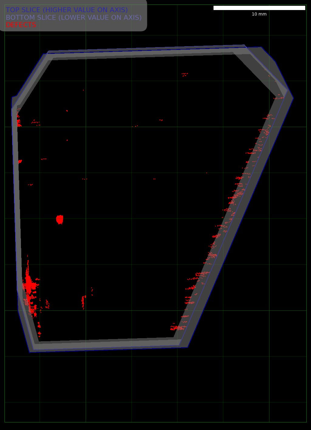
The output of this process is a set of images known as pre-processed plots (displayed on a black background).
Pre-processed plots: These images show the detected defects and the top and bottom slices of the crystal. The boundary slices are particularly helpful for checking differences in shape or size, ensuring that the cutting plan does not impact the outer edges of the crystal.
Grade Plots
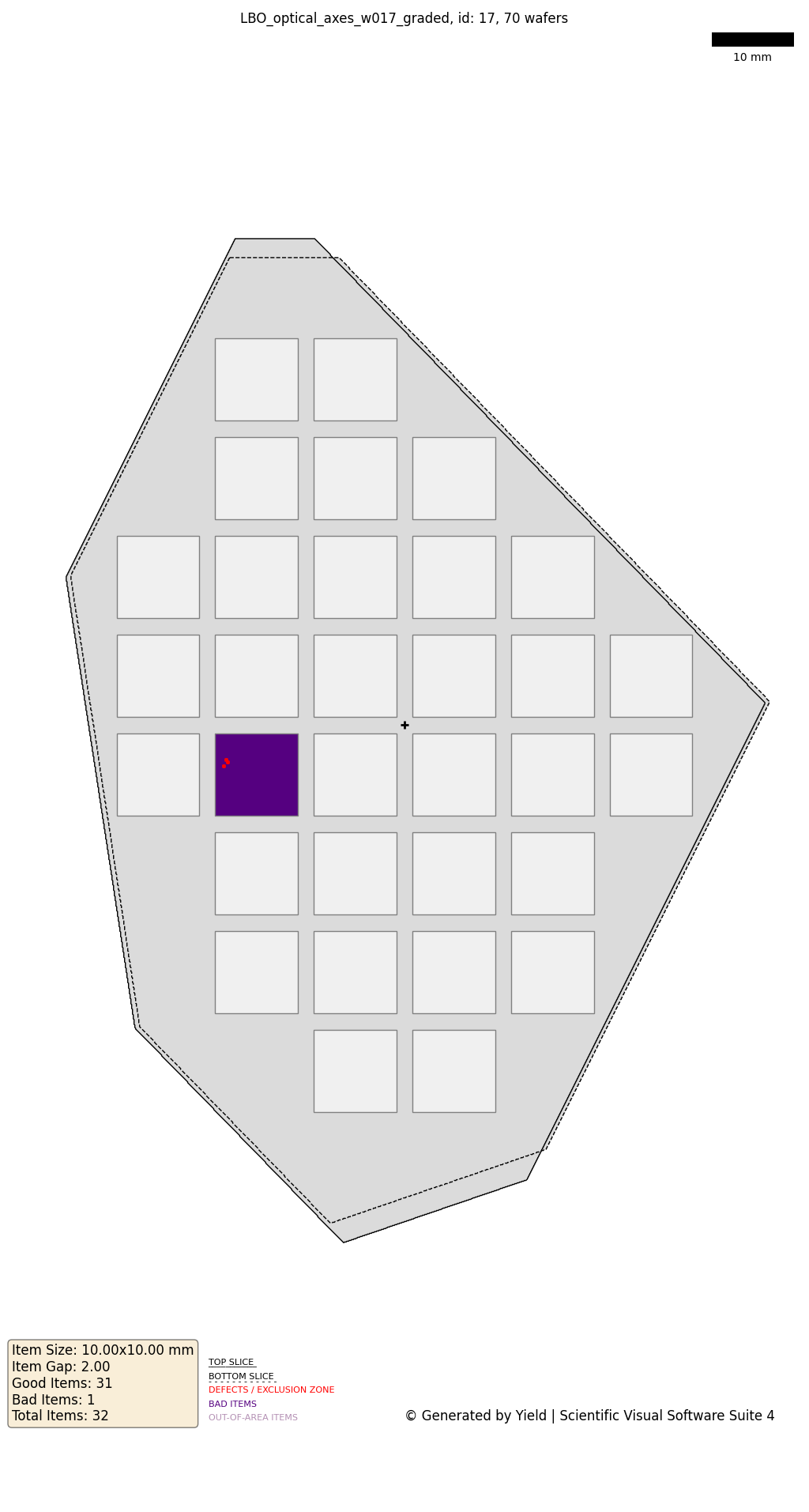
A graded plot is an image that visually represents the model's defects and potential cutting paths.
Important
You need to generate the plots before proceeding with grading.
How to Grade Plots?
Select Grade Plots... from the Tools menu in the top navigation bar. This will open a pop-up window with the following options:
Input Folder: Folder containing the generated plots to be graded.
Output Folder: Folder where the graded plots will be saved.
Item Shape: Chooses the shape of the items to be plotted. Options include Square or Rectangular. This setting determines how the items will be visualized in the plots.
Item Size: Size of the items to be plotted.
Item Gap: Distance between items in the plot.
Exclusion Zone: Defines a buffer zone around the crystal to avoid placing items too close to its edges.
You can also specify the following additional parameters, to optimize the positioning and orientation of the items in the plots:
Rotation Angle: The angle determines how the items are rotated in the plot. (Between 0 and 360 degrees)
Optimize Shift: If enabled, the algorithm will attempt to shift the items to optimize their placement within the plot. This can help maximize the number of items that fit within the defined area.
Press
Okbutton.
Example
General
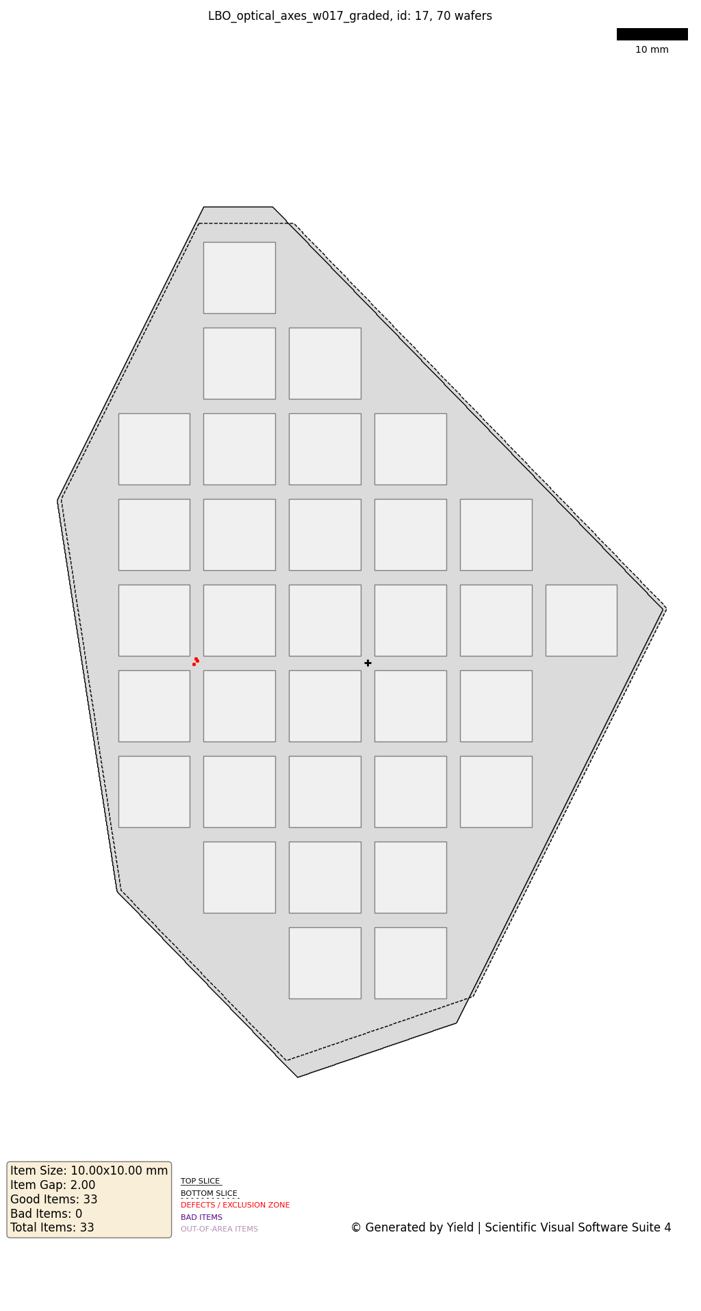
The following images display planned cutting paths (either square or rectangular) designed to optimize wafering or coring.

|

|
Optimized Shift vs. Non-Optimized Shift
The following images illustrate the difference between plots generated with and without the Optimize Shift option enabled.
The left image shows the result with the option disabled, while the right image shows the result with the option enabled.
|
|
Plots Key
Each plot contains a key, located on the top for black images and on the bottom for white images.
Pre-processed Plots
Red: Marks the defects present in the slice.
Dark Blue: Outlines the top slice border.
Light Blue: Represents the bottom of the slice.
Graded Plots
Solid Line: Represents the top of the slice.
Dashed Line: Represents the bottom of the slice.
Items on Plots
White: Defect-free items.
Green: the defect lies on the border of an item.
Brown: 1 defect.
Maroon: 2-3 defects.
Purple: Items with defects, labeled as 'bad'.
Light Purple: Indicates 'Out-of-area' items, these are items that either partially lie outside the crystal's border or are positioned too close to it. However, if the offset value is adjusted, the item might still be usable.